Reference Number	Description
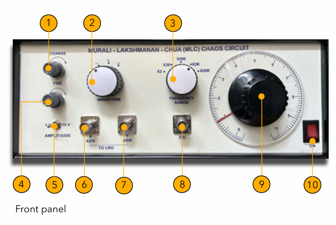
1	Coarse amplitude variation of input waveform F(t)
2	Input waveform F(t) selector knob: sine, triangular, square
3	Frequency range selector knob for input waveform F(t)
4	Fine variation of amplitude of input waveform F(t)
5	Amplitude range selector knob for input waveform F(t)
6	Output to CRO (x-axis) of the signal x(t)
7	Output to CRO (y-axis) of the signal y(t)
8	Output to CRO of the input waveform F(t)
9	Frequency selector dial of the input waveform F(t)
10	ON/OFF switch

The Murali-Lakshmanan-Chua (MLC) circuit is the simplest non-autonomous chaotic circuit that exhibits various complex dynamical behaviors under the influence of an external periodic signal. Cellular Neural Networks (CNNs) are a class of nonlinear dynamical systems that model various physical phenomena, including chaotic systems.

Researchers have embarked on a fascinating journey, exploring the implementation of the MLC circuit using standard forced LCR circuits with Chua’s diode or CNNs. In this groundbreaking approach, the dynamics of the MLC circuit are ingeniously modeled using a network of interconnected CNN cells. The CNN-based MLC circuit not only faithfully replicates the chaotic behavior of the original circuit but also offers the promising advantages of compactness, inductorless design, and ease of hardware implementation, igniting curiosity about its potential applications.

Key points about the MLC circuit:
MLC Circuit:

• A non-autonomous chaotic circuit
• Exhibits complex dynamical behaviors under external periodic forcing
• It can study various bifurcation sequences, chaotic structures, chaos control, and chaos synchronization.

CNNs:

• A class of nonlinear dynamical systems
• It can be used to model a variety of physical phenomena, including chaotic systems
• Offer advantages such as compactness and ease of hardware implementation.

CNN-based MLC Circuit:

• Models the dynamics of the MLC circuit using interconnected CNN cells
• It exhibits the same chaotic behavior as the original circuit
• Offers advantages in terms of compactness and ease of hardware implementation.

The original inductor based MLC circuit or inductor-less CNN-based MLC circuit holds immense potential for a variety of applications like secure communications, random number generation, chaos control, etc., inspiring researchers and engineers to explore its capabilities in depth.

References:

• K.Murali, M.Lakshmanan and L.O.Chua, “Bifurcation and chaos in the simplest dissipative non autonomous circuit”, Int.J.Bifurcation and Chaos 4, 1511-1524 (1994).
• M.Lakshmanan and K.Murali, "Experimental Chaos from Non-Autonomous Electronic Circuits”, Phil. Trans. R. Soc. London A 353, 33-46 (1995).
• M.Lakshmanan and K.Murali, “Chaos in Nonlinear Oscillators”, World Scientific, Singapore (1996).
• Enis Gunay, “MLC circuit in the frame of CNN”, Int.J.Bifurcation and Chaos 20, 3267-3274 (2010).

Murali – Lakshmanan – Chua (MLC) Chaos Circuit

Objective
To study the bifurcations and chaotic dynamics of Murali – Lakshmanan – Chua (MLC) circuit.

Apparatus and Materials

• Murali-Lakshmanan-Chua (MLC) chaos circuit kit
• Oscilloscope (1 Nos)
• CRO probes (BNC connectors) (2 Nos)

Background Information

Murali – Lakshmanan – Chua (MLC) circuit is a simple dissipative non-autonomous chaotic circuit which was introduced in 1994 [1-3]. This circuit contains the famous Chua’s diode as the only nonlinear element. Along with the Chua’s diode, the circuit contains a linear resistor, a linear inductor, a linear capacitor and a time-dependent periodic forcing signal (for example sine, triangular, square waves) generated from a function generator. The circuit configuration is depicted in Fig.1. It is a classic series type forced LCR circuit along with the nonlinear resistor (Chua’s diode, N) connected in parallel with the capacitor C. The experimental MLC circuit is shown in Fig.2. A typical bifurcation parameter is the forcing sinusoidal signal’s amplitude (A). By applying Kirchoff’s laws to the circuit of Fig. 1, the following coupled first-order differential equations are obtained:


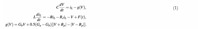
Here g(V) is the piecewise-linear function defined by Chua, et al [3] which is the mathematical representation of the characteristic curve of the Chua’s diode. The actual values of Ga, Gb and Bp are fixed as -0.76 ms, -0.41 ms and 1.0 V respectively.
SC-CNN BASED MLC CIRCUIT
State controlled-CNN (SC-CNN) is the CNN that can generate nonlinear dynamics, which was first introduced by arena et al. [4]. In that work, Chua circuit’s dynamics were imitated by a suitable connection of three CNN cells. Also, CNN-based Murali-Lakshmanan-Chua model (MLC) is performed by CNN cells[4]. This type of circuit attracts considerable interest due to its inductor less realisation. The SC-CNN-based MLC model is represented by
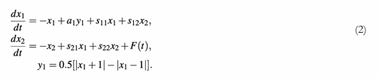
Here x1, x2 are the state variables (corresponding to X and Y variables in the circuit of Fig.3 and y1 is the nonlinear function. The SC-CNN parameters are fixed as: a1=0.47, s11=1.55, s12=1, s21 = -1, s22=-0.015 [4].

Experimental procedure

1. Connect the one end of the provided BNC cables to Channel-1 and Channel-2 of the dual channel oscilloscope. Connect the other ends of the BNC cables to terminals 6 and 7 respectively in the kit.
2. Connect the 230V India power plug (50Hz).
3. Switch ON the kit (Reference No.10)
4. Put the input WAVEFORM selector knob (Reference No.2) to sine wave.
5. Put the input waveform FREQUENCY RANGE selector knob (Reference No.3) to 2K position.
6. Put the input waveform frequency dial at 1 (Reference No. 9)
7. Put the AMPLITUDE of the input waveform control switch to 1V (Reference No.5)
8. Put the FINE variation knob (Reference No.4) to minimum.
9. Vary the COARSE variation know (Reference No.1) carefully in the kit until you observe a period-1 limit cycle (phase-portrait) in the oscilloscope as shown in Fig.4(a). Take a photo.
10. Increase slowly the COARSE knob until you observe a period-2 limit cycle in the oscilloscope as shown in Fig.4(b). Take a photo.
11. Now slowly vary the FINE knob (Reference 4) until you observe a period-4 limit cycle in the oscilloscope as shown in Fig.4(c). Take a photo.
12. Vary slowly the COARSE knob until you observe a single-band chaotic attractor in the oscilloscope as shown in Fig.4(d). Take a photo.
13. Vary slowly the COARSE knob until you observe a double-band chaotic attractor in the oscilloscope as shown in Fig.4(e). Take a photo.
14. Slowly increase the COARSE knob further to observe period-3 limit cycle, period-5 limit cycle and period-1 boundary.

Figures

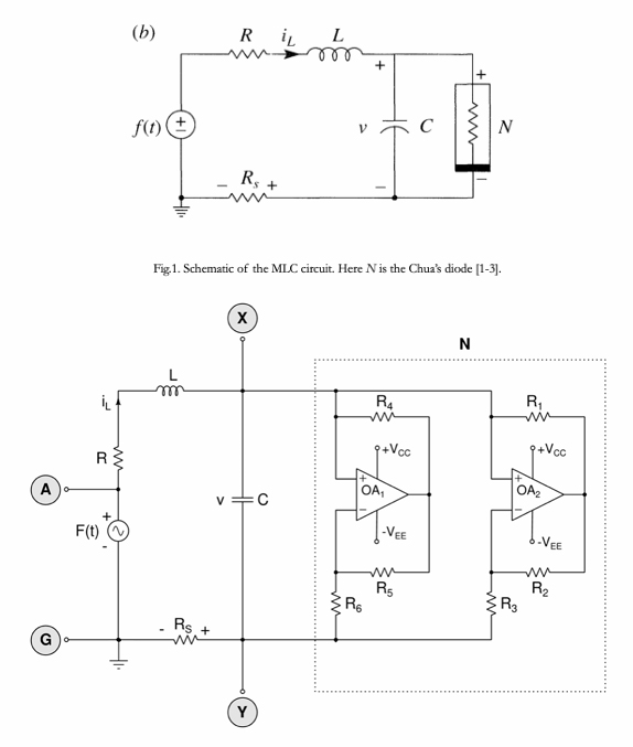
Fig.2. Experimental realization of the MLC circuit. The Chua’s diode (N) is realized with six resistors and two opamps OA1 and OA2. Here inductor L = 18 mH (TOKO type 10RB, Coilcraft type RFC0810B-186KE, or equivalent), Capacitor C = 10nF, Resistor R = 1340Ω, Resistors R1 = R2 = 220 Ω, R3 = 2.2 KΩ, R4 = R5 = 22 KΩ, and R6 = 3.3KΩ. The supply voltages are fixed as Vcc = +9V and VEE = -9V. The current sensing resistor Rs = 33Ω, The op-amps are AD712, µA741, TL082 or equivalent. The time varying input signal F(t) (sine, triangular or square wave) is generated by a function generator. The frequency of this signal is fixed as 8890 Hz. The amplitude of this signal is the control parameter to be varied to see the dynamical phenomena [1-3].


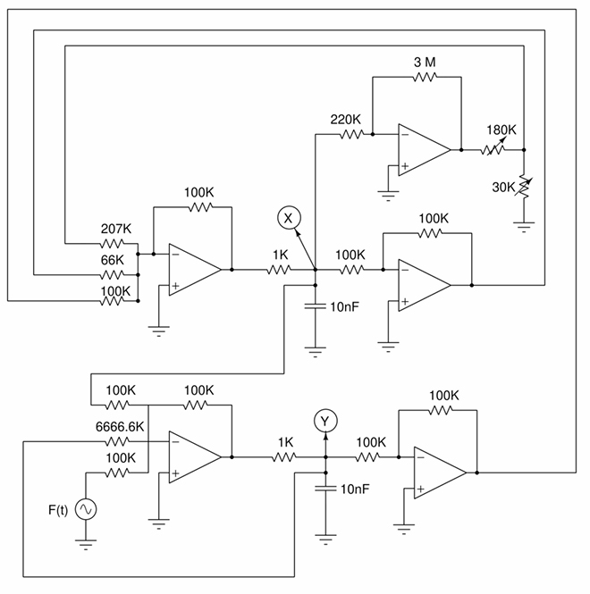
Fig. 3. Alternative experimental circuit realisation of Fig.2 based on CNN implementation. This circuit is used in the present kit for ease of operation and it is an inductor less realization. The op-amps are AD712, µA741, TL082 or equivalent. The time varying input signal (sine, triangular or square wave) is generated by a function generator F(t). The frequency of this signal is fixed as 2000 Hz. The amplitude (A) of this signal is the control parameter to be varied to observe the dynamical phenomena. Other parameters are used as shown in the figure. Two capacitors and five op-amps are used in this circuit. The supply voltages for the op-amps are fixed as Vcc = +9V and VEE = -9V [4].

Experimental Results
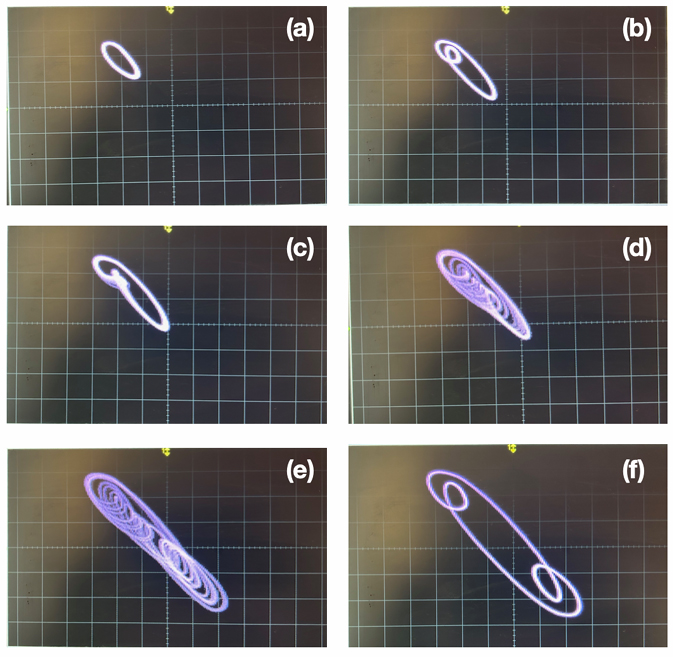
Fig.4. Typical bifurcation sequence in MLC circuit. Phase-portraits between voltages across two capacitors (X - Y) in Fig.3 are plotted. (a) Frequency of F(t) = 2KHz and amplitude, A =1.8Vpp, period-1 cycle; (b) A=2.0Vpp period-2 cycle; (c) A=2.2Vpp, period-4 cycle; d) A=3.2Vpp one-band chaos; (e) A=3.8Vpp, double-band chaos and (f) A = 4.0Vpp, period-3 cycle. Here x-axis 3V/div and y-axis 3V/div.

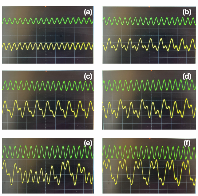
Fig.5. Typical bifurcation sequence in MLC circuit. Waveforms F(t) and x(t) are plotted. Upper trace F(t) and the bottom trace x(t). (a) Frequency of F(t) = 2KHz and amplitude, A =1.8Vpp, period-1; (b) A=2.0Vpp period-2; (c) A=2.2Vpp, period-4; d) A=3.2Vpp one-band chaos; (e) A=3.8Vpp, double-band chaos and (f) A = 4.0Vpp, period-3 cycle. Upper trace: 2V/div, bottom trace 5V/div and x-axis (time) 1ms/div.

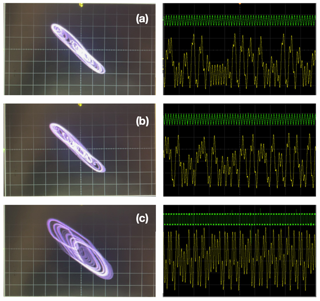
Fig.6. Phase-portraits (left panel) (X-axis: 5V/div and Y-axis: 5V/div) of double-band chaotic attractors for different periodic signals, F(t). The right panel: Top trace; The signal F(t) and the bottom trace is x(t) with Y-axis: 5.0V/div and time = 5.0ms./div. The frequency of F(t) is fixed as 2KHz. (a) F(t) = sine wave with amplitude, A = 3.0Vpp, (b) F(t) = triangular wave with amplitude, A=3.10Vpp (c) F(t) = square wave with Amplitude A = 4.3Vpp,

Precautions

Make sure the ground terminals of the kit and oscilloscope are properly connected.

Result

• Do not give too much AMPLITUDE of the input forcing signal.
• The chaotic dynamics of the Murali-Lakshmanan-Chua (MLC) circuit have been studied by varying the
• periodic forcing signal’s amplitude. Typical period-doubling route to chaos has been observed.

Exercises

1. By fixing the amplitude F of the sinusoidal forcing signal at a particular value and vary the forcing signal’s (F(t)) frequency and observe the typical different dynamical phenomena.
2. Try by putting the WAVEFORM selector knob to triangular or square waveforms and repeat the experiment to observe different dynamical phenomena including period-doubling bifurcations.
3. Try to connect one CRO BNC connector either X-axis terminal (Reference No.6) or Y-axis terminal (Reference No.7) to channel -1 and another CRO BNC connector to F(t) terminal (Reference No.8) to channel -2 of the oscilloscope and observe different phase-portraits by varying the amplitude or frequency of the input signal F(t).
4. Observe the time-waveforms of X-axis signal or Y-axis signal and compare it with the input signal F(t). Take a photo and analyse.

Questions

1. What is period-doubling bifurcation?
2. Is it possible to observe Poincare map of the strange attractor in oscilloscope?
3. Is it possible to design Chua’s diode with cubic nonlinearity?
4. What will happen to the period-doubling bifurcations to chaos in MLC circuit if it is driven by non- sinusoidal signals?
5. How the duty cycle of the square-wave input affect the dynamical phenomena of the present system?